In this tutorial, we’ll show you how to find and remove duplicates in your Excel document.
How to Find Duplicate Row or Data
It’s essential to first check which rows (or columns) have identical information. So before we show you how to remove duplicates in Excel, let’s walk you through the process of checking your sheet for duplicate data.
Method 1: Search Entire Worksheet
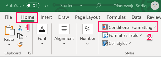
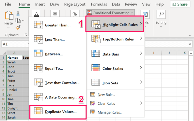
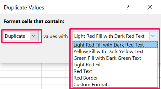
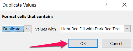
Excel has a Conditional Formatting tool that helps to identify, visualize, and draw conclusions from data. Here’s how to use the tool to highlight duplicate values in your Excel document. Excel will immediately highlight rows and columns with duplicate values.
Method 2: By Combining Rows
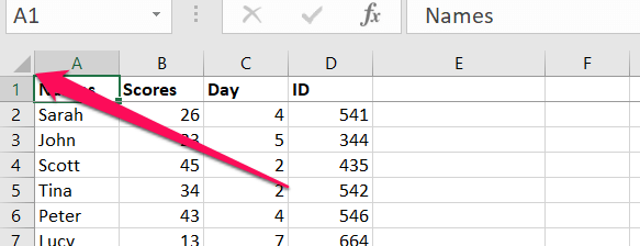
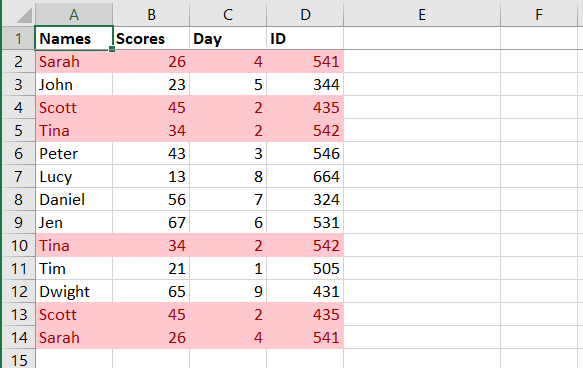
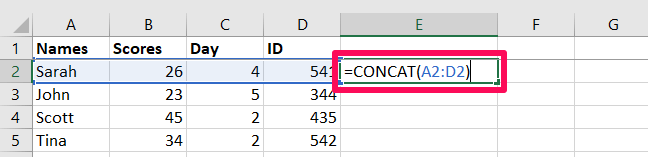
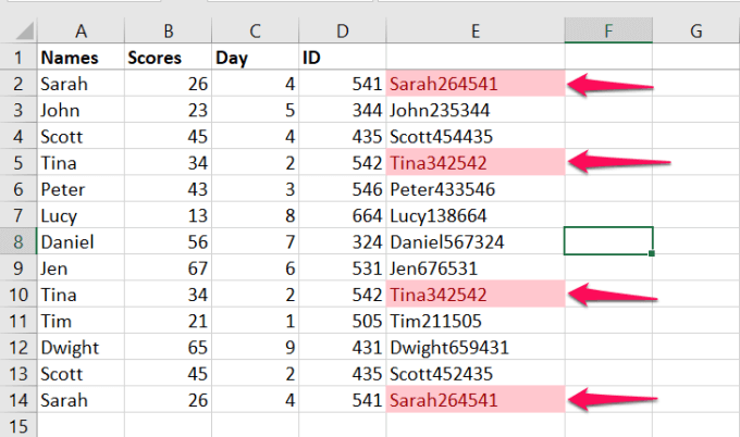
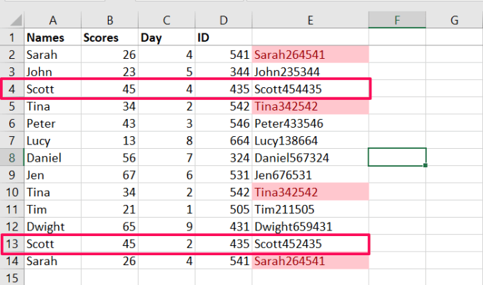
This method is perfect for finding rows with duplicate values across all columns or cells. First, you’ll need to use Excel’s “Concatenate” function to combine the content of each row. Then, select the column where you want the combined values stored and follow the steps below. We recommend combining the values in a column next to the last value on the first row. In our sample worksheet (see image below), the first and last cells on the first row have the reference A2 and D2, respectively. Hence, the formula will be this form: =CONCAT(A2:D2). Remember, the cell references will vary depending on the number of rows and columns on the table. Excel will highlight the column with duplicates values. That tells you to the cells in that particular row that have duplicate values as another row on the worksheet. If you look closely at the image above, you’ll notice that the Conditional Formatting tool did not highlight Row 4 and Row 13. Both rows have duplicate values in the Names, Scores, and ID columns, but different values in the Day column. Only 3 out of 4 columns in both rows have duplicate information. That explains why the Conditional Formatting tool didn’t highlight the concatenated or combined values for both rows. Both rows (Row 4 and Row 13) are unique because there’s distinguishing information in the “Day” column.
How to Remove Duplicate Rows in Excel
You’ve found multiple rows containing duplicate information in your Excel worksheet. Let’s show you how to remove these duplicate rows using two Excel tools.
1. Use the “Remove Duplicates” Tool
This tool has only one job: to ensure you have clean data in your Excel worksheet. It achieves this by comparing selected columns in your worksheet and removing rows with duplicate values. Here’s how to use the tool:
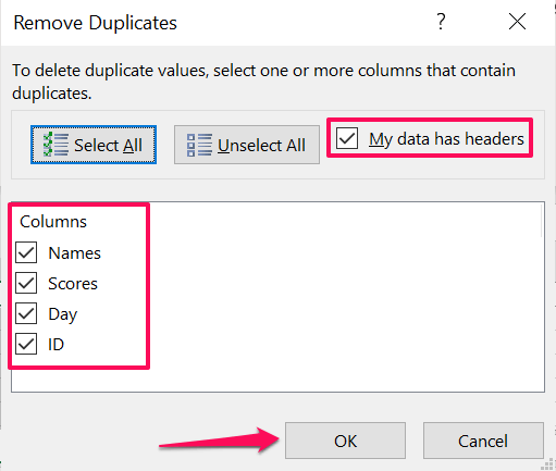
Select a cell on the table and press Control + A on your keyboard to highlight the table.
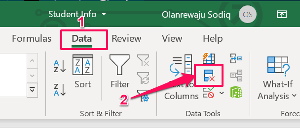
Go to the Data tab and click the Remove Duplicates icon in the “Data Tools” section.
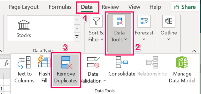
If your PC has a small screen or the Excel window is minimized, click the Data Tools drop-down button and select Remove Duplicates.
Go through the Columns section and select all columns. If your table has a header, check the box that reads “My data has headers.” That’ll deselect the header row or the first row on the sheet. Click OK to proceed.
Quick Tip: To make the first row of an Excel worksheet a header, go to the View tab, select Freeze Panes, and select Freeze Top Row.
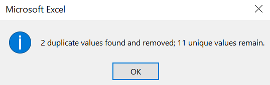
Excel will display a prompt notifying you of the total duplicate values found and removed from the sheet. Click OK to return to the worksheet.
2. Use the Advanced Filter Tool
“Advanced Filter” is another brilliant tool that helps you clean your data in Excel. The tool lets you view, edit, group and sort data on your worksheet. Follow the steps below to learn how to use this tool to remove duplicate rows from your Excel worksheet.
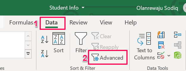
Select any cell on the table and press Control + A to highlight the entire table.
Go to the Data tab and select Advanced in the “Sort & Filter” section.
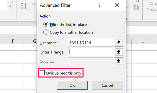
Check the Unique records only box and click OK.
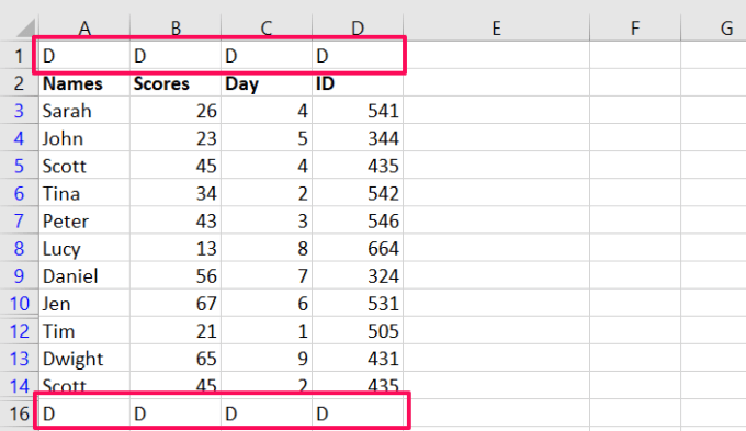
If the table or worksheet contains multiple rows with similar information or values, Excel will remove all but the first occurrence of the duplicates. Note: The Advanced Filter tool automatically treats the first row as a header. This means that the tool won’t remove the first row, even if it contains duplicate information. For instance, in the table below, running the “Unique records only” feature of the Advanced Filter tool did not remove the first and last rows—even though they both have duplicate values across all columns. So, if your Excel worksheet or table has a header, it’s best to use the “Remove Duplicates” tool to eliminate duplicate rows. Quick Tip: Removed duplicate rows or values by accident? Press Control + Z to revert the change and get back the duplicate data.
Removing Duplicates in Excel: Limitations
We should mention that you cannot remove duplicate rows or values from a worksheet containing outlined or grouped data. So if you grouped the rows and columns in your Excel worksheet, perhaps into Totals and Subtotals, you’ll have to ungroup the data before you can check for duplicates. Refer to this official documentation from Microsoft to learn more about removing duplicates in Excel and filtering unique values.